


Various word encoding methods like Integer/ Label Encoding or One-Hot Encoding have many limitations, among them, the main limitation is that these encoding doesn’t have the semantic relationship between the words. So, using these encodings, we have no way to find out that the words “Soccer” and “Football” are nearby words.
Also, In One-Hot Encoding, as vocabulary size increases, memory requirement increases, as well feature spaces increases. Feature space increase results in a curse of dimensionality issues. Whereas Integer/ Label Encoding suffers from undesirable bias.
We could use the WordNet list of Synonyms to get similarity, but it will fail due to the following issues:
- Many times, two words have the same meaning in some particular context only. Synonym list doesn’t contain that information
- We can define the synonyms of some limited combinations of words only, maintaining the list for all pairs of words is not possible. [suppose we have 1 million words in dictionary, then we would have to maintain the pair of 1 million * 1 million combinations. We can very well imagine what would happen in case we have 1 trillion words in our corpus.]
- As the vocabulary evolve, we need regularly update the synonym list
- It would be much more efficient and useful in case we can calculate the similarity between any two words by looking into their encoding.
So we should have some way where words can be encoded in low dimensionality space (predefined dimensions which are independent of vocab size) in such a way that similarity between two words can be calculated using this.
To achieve the above, the concept of embeddings has been introduced. Idea is to represent a word in a fixed vector space, which is not dependent on the size of the vocabulary. Using the vector representation of words, the similarity between two words can be calculated by calculating the distance of these two word’s vector representation, which is called embeddings.
In word embeddings, each word can be represented as an N-dimensional vector (mostly 300), and similarity between two words can be calculated by calculating the distance between these words in N-dimensional space. So, it solves the high dimensionality-related issues as well, which can be seen in One–Hot–Encoding where the dimension of word encoding increases as vocabulary size increases.
For calculating the word embeddings, intuition has been used that word’s meaning should be represented by the words that frequently appear nearby that word.
[“You shall know a word by the company it keeps” (J. R. Firth 1957: 11)]
Generating Word Embedding also evolve through various methodologies as below:
- SVD based methods
- Neural Network/ Iteration based methods
Initially, SVD based embeddings have been introduced. Using this method, first, we calculate word co-occurrence matrix based on Document Term Matrix or window-based Co-Occurrence Matrix. Then we reduce the dimensionality of the matrix using SVD, which gives the embeddings of each word in reduced space.
SVD based embeddings also suffer many limitations like word co-occurrence matrix very quickly become imbalance as the vocab size increases due to high-frequency words. Also, it has a very high training cost O(mn2) where m is the size of a vocabulary/ dictionary and n is the embedding size.
Here instead of computing the word embeddings as we have seen in SVD, the following Neural Network/ iterative Word Embedding based models are now becoming popular to calculate Word Embedding.
- Word2Vec
- GloVe
- fastText
In this blog, we will focus on Word2Vec, which was developed first compare to other models fastText and GloVe.
Word2Vec is developed by Google in 2013, whereas Glove by researchers from Stanford University in 2014 and fastText is developed by Facebook in 2015.
Word2Vec Embeddings
A team of Google researchers lead by Tomas Mikolov developed, patented, and published Word2Vec in two publications in 2013 (please refer to the Reference docs given at the end of the document). For learning word embeddings from raw text, Word2Vec is a computationally efficient predictive model.
Word2Vec is a shallow, two-layer neural network that is trained to reconstruct linguistic contexts of words. The idea is to design a model whose parameters are vectors. Then train the model on a certain objective. At every iteration we run our model, evaluate the errors, and follow an update rule.
It takes a large corpus of words as input and outputs a vector space with hundreds of dimensions, with each unique word in the corpus allocated to a corresponding vector in the space.
Word vectors are positioned in the vector space in such a way that words with similar contexts in the corpus are close together in the space.
It comes in two model architectures, the Continuous Bag-of-Words (CBOW) and the Skip-Gram. We will concentrate on Skip-Gram Architecture.
Word2Vec Skip-Gram Architecture:
In Skip-Gram architecture, the Objective of the model is to train the model in such a way so that given a central word our model should be able to predict the context words correctly.

Symbols Meaning:
 : input layer, which is one-hot encoding of center word
 : weight between the input layer and hidden layer
 : weight between the hidden layer and output layer
 : Vocabulary Size
 : Embedding Size/ Size of hidden layer
 : the hidden layer
 : Output layer before activation
 : Output layer after activation, predicted context words
 : Actual context words for center word x
 : Learning rate
 : Number of context words for a given center word
 : Number of training examples
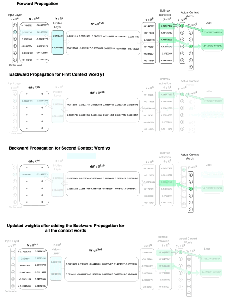
Forward Propagation:
![\[ h = W^T. x \]](https://gyan-mittal.com/wp-content/ql-cache/quicklatex.com-d23faeb5b7a67c30ee993ea3cb877b0b_l3.png "Rendered by QuickLaTeX.com")
![\[ u = W'^T.h\]](https://gyan-mittal.com/wp-content/ql-cache/quicklatex.com-1bfcaef0aa1ceb8bfd11e1126bf0b45d_l3.png "Rendered by QuickLaTeX.com")
![\[ \hat{y} = softmax(u)\]](https://gyan-mittal.com/wp-content/ql-cache/quicklatex.com-ec985a8c74c8289d64714884802cc703_l3.png "Rendered by QuickLaTeX.com")
Loss for every contxet word  for a given center word
![\[ J = -\sum_{w\in{V}} y_w.log(\hat{y_w}) = = - log(\hat{y_c}) \]](https://gyan-mittal.com/wp-content/ql-cache/quicklatex.com-d0d5383e93967be6fcef56b8b740fe66_l3.png "Rendered by QuickLaTeX.com")
Loss for all contxet words for a given center word is as following
![\[ J = - \sum_{c=1}^{C} log(\hat{y}_{c}) \]](https://gyan-mittal.com/wp-content/ql-cache/quicklatex.com-a05f6201ebc2842936ee2ce7b4ec10da_l3.png "Rendered by QuickLaTeX.com")
We have training examples and context words, the objective is to minimize following loss function:
![\[ J = - \frac{1}{T} \sum_{t=1}^{T} \sum_{c=1}^{C} log(\hat{y}_{t,c}) \]](https://gyan-mittal.com/wp-content/ql-cache/quicklatex.com-912b59694bb4a1645ec2f357412061ec_l3.png "Rendered by QuickLaTeX.com")
Backword Propogation:
![\[ \partial{J}/\partial{w'_{i,j}} = \sum_{c=1}^{C} (y_{c,j} - t_{c,j) \;. \;h_i \]](https://gyan-mittal.com/wp-content/ql-cache/quicklatex.com-ce9cb040861f55fbab0bf3b1a53cb414_l3.png "Rendered by QuickLaTeX.com")
![\[ \partial{J}/\partial{w_{k,i}} = \sum_{j=1}^{V} \sum_{c=1}^{C} (y_{c,j} - t_{c,j) \;. \;w'_{i,j} \;. \;x_k \]](https://gyan-mittal.com/wp-content/ql-cache/quicklatex.com-55537030799a7947c9f0d844be7ef47c_l3.png "Rendered by QuickLaTeX.com")
![\[ \;where\; t_{c,j}=1 \;if \;the \;j^{th} \;node \;of \;the \;c^{th} \;true \;output \;is \;1 \;else\; t_{c,j} = 0\]](https://gyan-mittal.com/wp-content/ql-cache/quicklatex.com-76579a29f4a4ece1cc963cd8164e8470_l3.png "Rendered by QuickLaTeX.com")
![\[ w_{i,j}^{'(new)} = w_{i,j}^{'(old)} - \alpha \;. \; \sum_{c=1}^{C} (y_{c,j} - t_{c,j) \;. \;h_i \]](https://gyan-mittal.com/wp-content/ql-cache/quicklatex.com-34135a674e16a81ef5292017bff0bfbf_l3.png "Rendered by QuickLaTeX.com")
![\[ w_{k,i}^{(new)} = w_{k,i}^{(old)} - \alpha \;. \; \sum_{j=1}^{V} \sum_{c=1}^{C} (y_{c,j} - t_{c,j) \;. \;w'_{i,j} \;. \;x_k \]](https://gyan-mittal.com/wp-content/ql-cache/quicklatex.com-7cb07e50a8d4638e8505a1b6912adfbb_l3.png "Rendered by QuickLaTeX.com")
After training the model, every row of W will correspond to word vector embedding of the corresponding word belongs to that row. Intuition is that weights of similar words would have similar embeddings as the would have the company of similar words.
To understand the skip-gram model, let us go through the following example.
Example of Word2Vec using Skip-Gram
In this example, the basic Word2Vec skip-gram model is explained without introducing any complex concept.
Let us consider that we have the following sentences in our different docs in the corpus:
Sentence1: I love playing Football
Sentence2: I love playing Cricket
Sentence3: I love playing sports
We are considering Embedding_size N as 2 in our example.
Vocabulary size V in the above example sentences is 6.
In our example sentence, our training data will look like the following with the window size 1:
| Sentence | Center Word (X_center_word_train) | Context Words (y_context_words_train) |
| Sentence1: I love playing Football | I | love |
| Sentence1: I love playing Football | love | I, Playing |
| Sentence1: I love playing Football | playing | love, Football |
| Sentence1: I love playing Football | Football | playing |
| Sentence2: I love playing Cricket | I | love |
| Sentence2: I love playing Cricket | love | I, playing |
| Sentence2: I love playing Cricket | playing | love, Cricket |
| Sentence2: I love playing Cricket | Cricket | playing |
| Sentence3: I love playing sports | I | love |
| Sentence3: I love playing sports | love | I, playing |
| Sentence3: I love playing sports | playing | love, sports |
| Sentence3: I love playing sports | sports | playing |
In this algorithm, we take the neural network of two layers. The objective of this neural network is to predict the context words, given the center word within a given window.
The first layer weights are of the size of Vocab_size * Embedding_size. Whereas the second layer weights size is Embedding_size * Vocab_size.
In the final layer, the softmax activation function is used to predict the context word.
Once the training is complete, then each row in the first layer weight becomes the embedding of the corresponding word index in the vocabulary.
This corpus has 6 unique words (vocabulary/ dictionary size)
vocabulary/ dictionary (Label/ Integer Encoding of Words): {‘i’: 0, ‘love’: 1, ‘playing’: 2, ‘football’: 3, ‘cricket’: 4, ‘sports’: 5}
Training data of above table, will now become as following:
X_train: [[1, 0, 0, 0, 0, 0], [0, 1, 0, 0, 0, 0], [0, 0, 1, 0, 0, 0], [0, 0, 0, 1, 0, 0], [1, 0, 0, 0, 0, 0], [0, 1, 0, 0, 0, 0], [0, 0, 1, 0, 0, 0], [0, 0, 0, 0, 1, 0], [1, 0, 0, 0, 0, 0], [0, 1, 0, 0, 0, 0], [0, 0, 1, 0, 0, 0], [0, 0, 0, 0, 0, 1]]
y_train: [[0, 1, 0, 0, 0, 0], [1, 0, 1, 0, 0, 0], [0, 1, 0, 1, 0, 0], [0, 0, 1, 0, 0, 0], [0, 1, 0, 0, 0, 0], [1, 0, 1, 0, 0, 0], [0, 1, 0, 0, 1, 0], [0, 0, 1, 0, 0, 0], [0, 1, 0, 0, 0, 0], [1, 0, 1, 0, 0, 0], [0, 1, 0, 0, 0, 1], [0, 0, 1, 0, 0, 0]]
Training data in table format along with corresponding word can be represented as follows:
| Sentence | Center Word (X_train) | Context Words (y_train) |
| Sentence1: I love playing Football | I [1, 0, 0, 0, 0, 0] | love [0, 1, 0, 0, 0, 0] |
| Sentence1: I love playing Football | love [0, 1, 0, 0, 0, 0] | I, Playing [1, 0, 1, 0, 0, 0] |
| Sentence1: I love playing Football | playing [0, 0, 1, 0, 0, 0] | love, Football [0, 1, 0, 1, 0, 0] |
| Sentence1: I love playing Football | Football [0, 0, 0, 1, 0, 0] | playing [0, 0, 1, 0, 0, 0] |
| Sentence2: I love playing Cricket | I [1, 0, 0, 0, 0, 0] | love [0, 1, 0, 0, 0, 0] |
| Sentence2: I love playing Cricket | love [0, 1, 0, 0, 0, 0] | I, playing [1, 0, 1, 0, 0, 0] |
| Sentence2: I love playing Cricket | playing [0, 0, 1, 0, 0, 0] | love, Cricket [0, 1, 0, 0, 1, 0] |
| Sentence2: I love playing Cricket | Cricket [0, 0, 0, 0, 1, 0] | playing [0, 0, 1, 0, 0, 0] |
| Sentence3: I love playing sports | I [1, 0, 0, 0, 0, 0] | love [0, 1, 0, 0, 0, 0] |
| Sentence3: I love playing sports | love [0, 1, 0, 0, 0, 0] | I, playing [1, 0, 1, 0, 0, 0] |
| Sentence3: I love playing sports | playing [0, 0, 1, 0, 0, 0] | love, sports [0, 1, 0, 0, 0, 1] |
| Sentence3: I love playing sports | sports [0, 0, 0, 0, 0, 1] | playing [0, 0, 1, 0, 0, 0] |
A the beginning we have the following weights initialized:
W:
[[ 0.17640523 0.04001572]
[ 0.0978738 0.22408932]
[ 0.1867558 -0.09772779]
[ 0.09500884 -0.01513572]
[-0.01032189 0.04105985]
[ 0.01440436 0.14542735]]
W‘:
[[ 0.07610377 0.0121675 0.04438632 0.03336743 0.14940791 -0.02051583]
[ 0.03130677 -0.08540957 -0.25529898 0.06536186 0.08644362 -0.0742165 ]]
In Our training example training data of first iteration is as following:
| Sentence | Center Word (X_train) | Context Words (y_train) |
| Sentence1: I love playing Football | I [1, 0, 0, 0, 0, 0] | love [0, 1, 0, 0, 0, 0] |
X: [1, 0, 0, 0, 0, 0]
y: [0, 1, 0, 0, 0, 0]

Concept to notice: h corresponds to the row of weights corresponding to the word index of training data. It means that every training data corresponds to a corresponding row of weight W. So after the training rows corresponding to similar words in W will have similar values. And the distance between two words can be calculated by calculating the distance between values of corresponding rows in W. So once training is completed then each row in W will become the embedding for the corresponding word that belongs to this index.
Similarly, training data of second iteration is as following:
| Sentence | Center Word (X_train) | Context Words (y_train) |
| Sentence1: I love playing Football | love [0, 1, 0, 0, 0, 0] | I, Playing [1, 0, 1, 0, 0, 0] |
X: [0, 1, 0, 0, 0, 0]
y: [1, 0, 1, 0, 0, 0]

Notice, now we have two context words.
Similarly we will train our model for remaining training set. This will be our one epoch. We have done this process in our training example for 1000 epochs. Summary of loss is as following:
epoch 0 loss = 2.7026976169578862 learning_rate_alpha: 0.001
epoch 100 loss = 2.68797227145197 learning_rate_alpha: 0.001
epoch 200 loss = 2.6731992825801623 learning_rate_alpha: 0.001
epoch 300 loss = 2.649735624190748 learning_rate_alpha: 0.001
epoch 400 loss = 2.603958412204618 learning_rate_alpha: 0.001
epoch 500 loss = 2.5125432210561343 learning_rate_alpha: 0.001
epoch 600 loss = 2.346991127035263 learning_rate_alpha: 0.001
epoch 700 loss = 2.109007118561944 learning_rate_alpha: 0.001
epoch 800 loss = 1.8655582377416664 learning_rate_alpha: 0.001
epoch 900 loss = 1.6800931978078923 learning_rate_alpha: 0.001
epoch 999 loss = 1.5545440269879862 learning_rate_alpha: 0.001
Updated value of weight W after 1000 epochs of training:
[[ 1.149124 -0.86998417]
[-0.04047704 1.48333981]
[ 0.55466348 -0.8665634 ]
[ 0.02787687 0.25416947]
[-0.06727489 0.29595964]
[-0.03852687 0.38587039]]
After training the model, every row of W will correspond to word vector embedding of the corresponding word belongs to that row. So our embedding for each word after 1000 epochs looks as following:
| Word Index | Word | Embedding-> | |
| 0 | i | 1.149123999 | -0.8699841668 |
| 1 | love | -0.04047703988 | 1.483339811 |
| 2 | playing | 0.5546634793 | -0.8665633952 |
| 3 | football | 0.02787686912 | 0.2541694707 |
| 4 | cricket | -0.06727488884 | 0.2959596391 |
| 5 | sports | -0.03852687391 | 0.3858703899 |
Embeddings after 1000 epochs are as following:

You can notice that since in our example sports, cricket and football are used in the same context, so their embeddings are nearby compared to other words once training gets completed.
Word Embeddings in 2-D space and training loss can be represented as follows after each epoch:

Please observe in the above that how the embeddings of each word are converging after each epoch and Loss is getting reduced.
Limitations
In this blog, we have covered the naive implementation of the Word2Vec Skip-Gram model. Training time and memory requirements will quickly increase as soon as our vocab size increases.
To overcome the above limitations Word2Vec paper suggests trying the following improvements:
- Using Hierarchical Softmax instead of softmax
- Use negative sampling
Also, the paper suggests the Subsampling of Frequent Words so that frequent words like “in”, “the”, and “a” etc., which usually provide less information compared to other words can be removed from the training.
Further Work
We have just gone through the naive implementation of the Word2Vec Skip-Gram model in this blog. For now, we are parking the detailed discussion on improvements suggested to the naive Skip-Gram Word2vec implementation for some later days. Similarly, We will try to cover the Word2Vec CBOW model and which model is more suited in which situation.
We will also try to cover a detailed discussion of models like fastText, and GloVe including differences and improvements with comparison to other models.
Python code of the above Example for Document Term Matrix (GitHub code location) is as follows:
'''
Author: Gyan Mittal
Corresponding Document: https://gyan-mittal.com/nlp-ai-ml/nlp-word2vec-skipgram-neural-network-iteration-based-methods-word-embeddings
Brief about word2vec: A team of Google researchers lead by Tomas Mikolov developed, patented, and published Word2vec in two publications in 2013.
For learning word embeddings from raw text, Word2Vec is a computationally efficient predictive model.
Word2Vec methodology is used to calculate Word Embedding based on Neural Network/ iterative.
Word2Vec methodology have two model architectures: the Continuous Bag-of-Words (CBOW) model and the Skip-Gram model.
About Code: This code demonstrates the basic concept of calculating the word embeddings
using word2vec methodology using Skip-Gram model.
'''
from collections import Counter
import itertools
import numpy as np
import re
import matplotlib.pyplot as plt
import os
import imageio
# Clean the text after converting it to lower case
def naive_clean_text(text):
text = text.strip().lower() #Convert to lower case
text = re.sub(r"[^A-Za-z0-9]", " ", text) #replace all the characters with space except mentioned here
return text
def naive_softmax(x):
exp_x = np.exp(x)
return exp_x / exp_x.sum()
def prepare_training_data(corpus_sentences):
window_size = 1
split_corpus_sentences_words = [naive_clean_text(sentence).split() for sentence in corpus_sentences]
X_center_word_train = []
y_context_words_train = []
word_counts = Counter(itertools.chain(*split_corpus_sentences_words))
vocab_word_index = {x: i for i, x in enumerate(word_counts)}
reverse_vocab_word_index = {value: key for key, value in vocab_word_index.items()}
vocab_size = len(vocab_word_index)
for sentence in split_corpus_sentences_words:
for i in range(len(sentence)):
center_word = [0 for x in range(vocab_size)]
center_word[vocab_word_index[sentence[i]]] = 1
context = [0 for x in range(vocab_size)]
for j in range(i - window_size, i + window_size+1):
#print(i, "\t", j)
if i != j and j >= 0 and j < len(sentence):
context[vocab_word_index[sentence[j]]] = 1
X_center_word_train.append(center_word)
y_context_words_train.append(context)
return X_center_word_train, y_context_words_train, vocab_word_index
def naive_softmax_loss_and_gradient(h, context_word_idx, W1):
u = np.dot(W1.T, h)
yhat = naive_softmax(u)
loss_context_word = -np.log(yhat[context_word_idx])
#prediction error
e = yhat.copy()
e[context_word_idx] -= 1
dW_context_word = np.dot(W1, e)
dW1_context_word = np.dot(h[:, np.newaxis], e[np.newaxis, :])
return loss_context_word, dW_context_word, dW1_context_word
def plot_embeddings_and_loss(W, vocab_word_index, loss_log, epoch, max_loss, img_files=[]):
fig, (ax1, ax2) = plt.subplots(1, 2, sharex=False, figsize=(10, 5))
ax1.set_title('Word Embeddings in 2-d space for the given example')
plt.setp(ax1, xlabel='Embedding dimension - 1', ylabel='Embedding dimension - 2')
#ax1.set_xlim([min(W[:, 0]) - 1, max(W[:, 0]) + 1])
#ax1.set_ylim([min(W[:, 1]) - 1, max(W[:, 1]) + 1])
#ax1.set_xlim([-3, 3.5])
#ax1.set_ylim([-3.5, 3])
for word, i in vocab_word_index.items():
x_coord = W[i][0]
y_coord = W[i][1]
ax1.plot(x_coord, y_coord, "cD", markersize=5)
ax1.text(x_coord, y_coord, word, fontsize=10)
ax2.set_title("Loss graph")
plt.setp(ax2, xlabel='#Epochs (Log scale)', ylabel='Loss')
ax2.set_xlim([1 , epoch * 1.1])
ax2.set_xscale('log')
ax2.set_ylim([0, max_loss * 1.1])
if(len(loss_log) > 0):
ax2.plot(1, max(loss_log), "bD")
ax2.plot(loss_log, "b")
ax2.set_title("Loss is " + r"![\bf{" + str("{:.6f}".format(loss_log[-1])) + "}](https://gyan-mittal.com/wp-content/ql-cache/quicklatex.com-736d19406cdadfe3528d5e6c0f66b2d9_l3.png "Rendered by QuickLaTeX.com") " + " after " + r"
" + " after " + r" " + " epochs")
directory = "images"
if not os.path.exists(directory):
os.makedirs(directory)
filename = f'images/{len(loss_log)}.png'
for i in range(13):
img_files.append(filename)
# save frame
plt.savefig(filename)
plt.close()
return img_files
def create_gif(input_image_filenames, output_gif_name):
# build gif
with imageio.get_writer(output_gif_name, mode='I') as writer:
for image_file_name in input_image_filenames:
image = imageio.imread(image_file_name)
writer.append_data(image)
# Remove image files
for image_file_name in set(input_image_filenames):
os.remove(image_file_name)
def train(x_train, y_train, vocab_word_index, embedding_dim=2, epochs=1000, learning_rate_alpha=1e-03):
vocab_size = len(vocab_word_index)
loss_log = []
saved_epoch_no = 0
np.random.seed(0)
W = np.random.normal(0, .1, (vocab_size, embedding_dim))
W1 = np.random.normal(0, .1, (embedding_dim, vocab_size))
for epoch_number in range(0, epochs):
loss = 0
for i in range(len(x_train)):
dW = np.zeros(W.shape)
dW1 = np.zeros(W1.shape)
h = np.dot(W.T, x_train[i])
for context_word_idx in range(vocab_size):
if (y_train[i][context_word_idx]):
loss_context_word, dW_context_word, dW1_context_word = naive_softmax_loss_and_gradient(h, context_word_idx, W1)
loss += loss_context_word
current_center_word_idx = -1
for c_i in range(len(x_train[i])):
if x_train[i][c_i] == 1:
current_center_word_idx = c_i
break
dW[current_center_word_idx] += dW_context_word
dW1 += dW1_context_word
W -= learning_rate_alpha * dW
W1 -= learning_rate_alpha * dW1
loss /= len(x_train)
if (epoch_number == 0):
image_files = plot_embeddings_and_loss(W, vocab_word_index, loss_log, epochs, loss)
loss_log.append(loss)
loss_log.append(loss)
if(epoch_number%(epochs/10) == 0 or epoch_number == (epochs - 1) or epoch_number == 0):
print("epoch ", epoch_number, " loss = ", loss, " learning_rate_alpha:\t", learning_rate_alpha)
if ((epoch_number == 1) or np.ceil(np.log10(epoch_number + 2)) > saved_epoch_no or (epoch_number + 1) == epochs):
image_files = plot_embeddings_and_loss(W, vocab_word_index, loss_log, epochs, max(loss_log), image_files)
saved_epoch_no = np.ceil(np.log10(epoch_number + 2))
return W, W1, image_files
def plot_embeddings(W, vocab_word_index):
for word, i in vocab_word_index.items():
x_coord = W[i][0]
y_coord = W[i][1]
plt.scatter(x_coord, y_coord)
plt.annotate(word, (x_coord, y_coord))
print(word, ":\t[", x_coord, ",", y_coord, "]")
plt.show()
embedding_dim = 2
epochs = 2000
learning_rate_alpha = 1e-03
corpus_sentences = ["I love playing Football", "I love playing Cricket", "I love playing sports"]
#corpus_sentences = ["I love playing Football"]
x_train, y_train, vocab_word_index = prepare_training_data(corpus_sentences)
W, W1, image_files = train(x_train, y_train, vocab_word_index, embedding_dim, epochs, learning_rate_alpha)
print("W1:\t", W1, W1.shape)
print("W:\t", W, W.shape)
create_gif(image_files, 'images/word2vec_skipgram.gif')
" + " epochs")
directory = "images"
if not os.path.exists(directory):
os.makedirs(directory)
filename = f'images/{len(loss_log)}.png'
for i in range(13):
img_files.append(filename)
# save frame
plt.savefig(filename)
plt.close()
return img_files
def create_gif(input_image_filenames, output_gif_name):
# build gif
with imageio.get_writer(output_gif_name, mode='I') as writer:
for image_file_name in input_image_filenames:
image = imageio.imread(image_file_name)
writer.append_data(image)
# Remove image files
for image_file_name in set(input_image_filenames):
os.remove(image_file_name)
def train(x_train, y_train, vocab_word_index, embedding_dim=2, epochs=1000, learning_rate_alpha=1e-03):
vocab_size = len(vocab_word_index)
loss_log = []
saved_epoch_no = 0
np.random.seed(0)
W = np.random.normal(0, .1, (vocab_size, embedding_dim))
W1 = np.random.normal(0, .1, (embedding_dim, vocab_size))
for epoch_number in range(0, epochs):
loss = 0
for i in range(len(x_train)):
dW = np.zeros(W.shape)
dW1 = np.zeros(W1.shape)
h = np.dot(W.T, x_train[i])
for context_word_idx in range(vocab_size):
if (y_train[i][context_word_idx]):
loss_context_word, dW_context_word, dW1_context_word = naive_softmax_loss_and_gradient(h, context_word_idx, W1)
loss += loss_context_word
current_center_word_idx = -1
for c_i in range(len(x_train[i])):
if x_train[i][c_i] == 1:
current_center_word_idx = c_i
break
dW[current_center_word_idx] += dW_context_word
dW1 += dW1_context_word
W -= learning_rate_alpha * dW
W1 -= learning_rate_alpha * dW1
loss /= len(x_train)
if (epoch_number == 0):
image_files = plot_embeddings_and_loss(W, vocab_word_index, loss_log, epochs, loss)
loss_log.append(loss)
loss_log.append(loss)
if(epoch_number%(epochs/10) == 0 or epoch_number == (epochs - 1) or epoch_number == 0):
print("epoch ", epoch_number, " loss = ", loss, " learning_rate_alpha:\t", learning_rate_alpha)
if ((epoch_number == 1) or np.ceil(np.log10(epoch_number + 2)) > saved_epoch_no or (epoch_number + 1) == epochs):
image_files = plot_embeddings_and_loss(W, vocab_word_index, loss_log, epochs, max(loss_log), image_files)
saved_epoch_no = np.ceil(np.log10(epoch_number + 2))
return W, W1, image_files
def plot_embeddings(W, vocab_word_index):
for word, i in vocab_word_index.items():
x_coord = W[i][0]
y_coord = W[i][1]
plt.scatter(x_coord, y_coord)
plt.annotate(word, (x_coord, y_coord))
print(word, ":\t[", x_coord, ",", y_coord, "]")
plt.show()
embedding_dim = 2
epochs = 2000
learning_rate_alpha = 1e-03
corpus_sentences = ["I love playing Football", "I love playing Cricket", "I love playing sports"]
#corpus_sentences = ["I love playing Football"]
x_train, y_train, vocab_word_index = prepare_training_data(corpus_sentences)
W, W1, image_files = train(x_train, y_train, vocab_word_index, embedding_dim, epochs, learning_rate_alpha)
print("W1:\t", W1, W1.shape)
print("W:\t", W, W.shape)
create_gif(image_files, 'images/word2vec_skipgram.gif')
Thanks for your blog, nice to read. Do not stop.
Thanks Mark